Parametrization of an ODE coefficient

[facundoroffet]

Hi, I’m trying to solve a system of two coupled equations. The system (the Hopf oscillator), has two coefficients: a and w. I have succesfully trained a model capable of solve the system for a=0.6 and w=1, but now I want to parameterize it with respect to a in the range (-1,1).
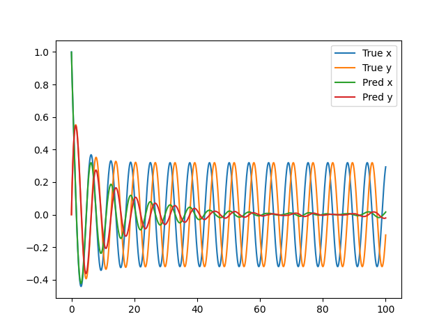
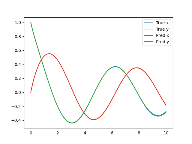
Following a tutorial (Parameterized 3D Heat Sink - NVIDIA Docs), I’ve modified my scripts to add the parameterization but it seem like I’m not getting the desired output.
Can someone tell me what I’m doing wrong? And also, how can I plot the results?

class Hopf(PDE):
    name = "Hopf"

    def __init__(self, a=0.6, w=1):
        self.a = a
        self.a = w

        t = Symbol("t")
        input_variables = {"t": t}

        x = Function("x")(*input_variables)
        y = Function("y")(*input_variables)

        if type(a) is str:
            a = Function(a)(*input_variables)
        elif type(a) in [float, int]:
            a = Number(a)
        if type(w) is str:
            w = Function(w)(*input_variables)
        elif type(w) in [float, int]:
            w = Number(w)

        self.equations = {}
        self.equations["ode_x"] = x.diff(t)-(a*x - w*y - x*(x**2 + y**2))
        self.equations["ode_y"] = y.diff(t)-(a*y + w*x - y*(x**2 + y**2))

@modulus.sym.main(config_path="conf", config_name="config")
def run(cfg: ModulusConfig) -> None:
    # make list of nodes to unroll graph on
    a, w = 0.6, 1
    hopf = Hopf(a=a, w=w)
    hopf_net = instantiate_arch(
        input_keys=[Key("t"), Key("a")],
        output_keys=[Key("x"), Key("y")],
        cfg=cfg.arch.fully_connected,
        activation_fn=Activation.SIN
    )
    nodes = hopf.make_nodes() + [hopf_net.make_node(name="hopf_network")]

    # add constraints to solver
    # make geometry
    geo = Point1D(0)
    t_min = 0.0
    t_max = 20.0
    t_symbol = Symbol("t")
    a_symbol = Symbol("a")
    x = Symbol("x")
    y = Symbol("y")
    time_range = {t_symbol: (t_min, t_max)}

    ic_param = {t_symbol: 0, a_symbol: (-1.0, 1.0)}
    initial_param = {t_symbol: (t_min, t_max), a_symbol: (-1.0, 1.0)}

    # make domain
    domain = Domain()

    # initial conditions
    IC = PointwiseBoundaryConstraint(
        nodes=nodes,
        geometry=geo,
        outvar={"x": 1.0, "y": 0},
        batch_size=cfg.batch_size.IC,
        # parameterization={t_symbol: 0},
        parameterization=ic_param,
    )
    domain.add_constraint(IC, name="IC")

    # solve over given time period
    interior = PointwiseBoundaryConstraint(
        nodes=nodes,
        geometry=geo,
        outvar={"ode_x": 0.0, "ode_y": 0.0},
        batch_size=cfg.batch_size.interior,
        # parameterization=time_range,
        parameterization=initial_param,
    )
    domain.add_constraint(interior, "interior")  

    # make solver
    slv = Solver(cfg, domain)

    # start solver
    slv.solve()

Thank you!

[ngeneva]

Hi @facundoroffet

Thanks for trying out Modulus. Glad you’ve got the non-parameterized version working! Parameterized solutions can be a lot more tricky but much more useful in the end.

I’ve modified my scripts to add the parameterization but it seem like I’m not getting the desired output. Can someone tell me what I’m doing wrong?

Can you elaborate by what you mean here? For example, Is the convergence bad? Is it unstable? Just not running?

And also, how can I plot the results?

Add a inferencer or validator (for example in the annular ring problem). Additional post processing information in the Modulus-Sym docs!

[facundoroffet]

Hi, thank you for your answer!

I wasn’t sure what the problem was, but then I realized that the parameterization wasn’t doing anything (the model was still being trained for one value of ‘a’).

But luckily, I was able to fix the code, so now everything is working as intended. Below I show the full code in case anyone finds it useful.

class Hopf(PDE):
    name = "Hopf"

    def __init__(self, w=1):
        self.a = w

        t = Symbol("t")
        a = Symbol("a")
        input_variables = {"t": t, "a": a}

        x = Function("x")(*input_variables)
        y = Function("y")(*input_variables)

        if type(w) is str:
            w = Function(w)(*input_variables)
        elif type(w) in [float, int]:
            w = Number(w)

        self.equations = {}
        self.equations["ode_x"] = x.diff(t)-(a*x - w*y - x*(x**2 + y**2))
        self.equations["ode_y"] = y.diff(t)-(a*y + w*x - y*(x**2 + y**2))

@modulus.sym.main(config_path="conf", config_name="config")
def run(cfg: ModulusConfig) -> None:
    
    # instantiate ode and network
    hopf = Hopf()
    hopf_net = instantiate_arch(
        input_keys=[Key("t"), Key("a")],
        output_keys=[Key("x"), Key("y")],
        cfg=cfg.arch.fully_connected,
        activation_fn=Activation.SIN
    )
    
    # make list of nodes to unroll graph on
    nodes = hopf.make_nodes() + [hopf_net.make_node(name="hopf_network")]

    # make geometry
    geo = Point1D(0)
    
    # create variables
    x, y = Symbol("x"), Symbol("y")
    
    # create parameters
    a = Symbol("a")
    a_range = (cfg.custom.a_min, cfg.custom.a_max)
    a_samples = cfg.custom.a_samples
    
    # define time
    t_min, t_max = cfg.custom.t_min, cfg.custom.t_max
    t = Symbol("t")
    t_range = (t_min, t_max)
    
    # initial conditions
    x_0 = 1.0
    y_0 = 0.0

    # make ranges
    ic_param_ranges = {t: 0, a: a_range}
    interior_param_ranges = {t: t_range, a: a_range}

    # make domain
    domain = Domain()

    # initial conditions
    IC = PointwiseBoundaryConstraint(
        nodes=nodes,
        geometry=geo,
        outvar={"x": x_0, "y": y_0},
        batch_size=cfg.batch_size.IC,
        parameterization=Parameterization(ic_param_ranges),
    )
    domain.add_constraint(IC, name="IC")

    # solve over given time period
    interior = PointwiseBoundaryConstraint(
        nodes=nodes,
        geometry=geo,
        outvar={"ode_x": 0.0, "ode_y": 0.0},
        batch_size=cfg.batch_size.interior,
        parameterization=Parameterization(interior_param_ranges),
    )
    domain.add_constraint(interior, "interior")

    # for scipy solution
    def ode(t, vars, a=0.6, w=1):
        x, y = vars
        dxdt = a*x - w*y - x*(x**2 + y**2)
        dydt = a*y + w*x - y*(x**2 + y**2)
        return [dxdt, dydt] 
    deltaT = 0.001
    t_scipy = np.arange(t_min, t_max, deltaT)  

    # create data for each param value
    values_a = np.linspace(*a_range, a_samples)
    for sample_a in values_a:
        sample_a = float(sample_a)
        specific_param_ranges = {
            a: sample_a,
        }

        # add metrics for front pressure
        geo_param_ranges = {
            **specific_param_ranges,
        }

        sol = solve_ivp(partial(ode, a=sample_a), (t_min, t_max), [x_0, y_0], t_eval=t_scipy)
        invar_numpy = {
            "t": np.expand_dims(t_scipy, axis=-1),
            "a": np.full_like(np.expand_dims(t_scipy, axis=-1), sample_a)
        }
        outvar_numpy = {
            "x": np.expand_dims(sol.y[0].T, axis=-1),
            "y": np.expand_dims(sol.y[1].T, axis=-1),
        }
                    
        validator = PointwiseValidator(
            nodes=nodes, invar=invar_numpy, true_outvar=outvar_numpy, batch_size=1024
        )
        domain.add_validator(validator)  

        print(sample_a)

    # make solver
    slv = Solver(cfg, domain)

    # start solver
    slv.solve()


if __name__ == "__main__":
    run()

[facundoroffet]

I think now I’m having another problem.

I trained a model for ‘a’ in the range [-0.1, 0.1], and got a small loss (≈2e-5). But the results differ a lot from the reference solutions.

For a=0.1:

Is there something that I’m still doing wrong?

[ngeneva]

Hi @facundoroffet

This looks like a convergence problem. Its likely the (wrong) prediction does satisfy the PDE loss in some loose form so the error appears small. Consider trying weighting your ODE loss constraint more via the lambda weighting parameter, modifying your network, train more on the earlier time steps than the later or some of the tricks we mention in our user guide.

Personally I would start training a smaller time range (say 0 - 10) and see if it can converge there. If so you know your loss is working, its a matter of how you train it for longer roll outs.

[facundoroffet]

Thank you a lot for the help!! I tried what you suggested: I got the same loss (≈2e-5), but now the results are very good. For a=0.1:

Any tips regarding how to train the model for longer? Because the results are already starting to get worse when I train it for the range 0-20.

[ngeneva]

Hi @facundoroffet

Long time predictions is where a lot of experimentation is often required.

• You may have to slowly unroll to longer time scales
• Consider trying some of the other models we support such as the Fourier Networks.
• Are you scaling your time range? Typically a range from 0 to 100 would lead to problems for a neural network.
• May need to train for a longer time with more training points.
• Etc.

Also have a browse of the Recommended Practices section of the docs for some tricks to consider. Good luck!